

2021 THEMIS SCIENCE NUGGETS
Estimating Precipitating Energy Flux, Average Energy, and Hall Auroral Conductance from THEMIS All-Sky-Imagers with Focus on Mesoscales
by Christine Gabrielse
The Aerospace Corporation
Introduction
The aurora provides a dazzling, dynamic display of colors across the night sky. During substorms, the aurora can span across all of Canada, making the entire process impossible to view from one observer's location. As one might expect, such a dynamic event deposits a lot of energy from the magnetosphere into Earth's ionosphere, which has effects even into the thermosphere (e.g., Deng et al., 2019). The precipitating energetic particles behind the aurora also heat the upper atmosphere, causing upwelling and increased drag on low-orbiting satellites and the International Space Station. To understand where and how this energy is deposited, scientists have relied upon statistics and empirical models of satellite overpasses-since satellites can obtain a 2D picture but are not stationed over the same location and therefore cannot view the evolution of a substorm aurora (e.g., Newell, Sotirelis, & Wing, 2010; Newell, Sotirelis, Liou, et al., 2010; Newell, Lee, et al., 2010; Zhu, Deng, et al., 2021; McGranaghan et al., 2021). Scientists have also used imagers on satellites that have a larger view (e.g., Burch et al., 2001; Liou, K. , 2010), but these imagers could not resolve meso- or small-scales. Ground-based instrumentation has also been employed, but as mentioned, one instrument can only see what occurs above it and will miss the auroral evolution at different locations (e.g., Partamies et al., 2004; Kauristie et al., 2006). The mosaic of THEMIS all-sky-imagers (ASIs) solves these observational issues by providing a large array with a combined field-of-view that spans all of Canada and Alaska, while being stationary and therefore able to view the auroral evolution over time for hours on end (Mende et al., 2008). We utilized the THEMIS ASIs in concert with meridian-scanning photometers to design a new technique that allows us to estimate the auroral energy flux, average energy, and resulting conductance. The THEMIS ASI resolution allows us to constrain these parameters to mesoscales (<500 km wide) with temporal resolution as fine as 3 seconds.
|
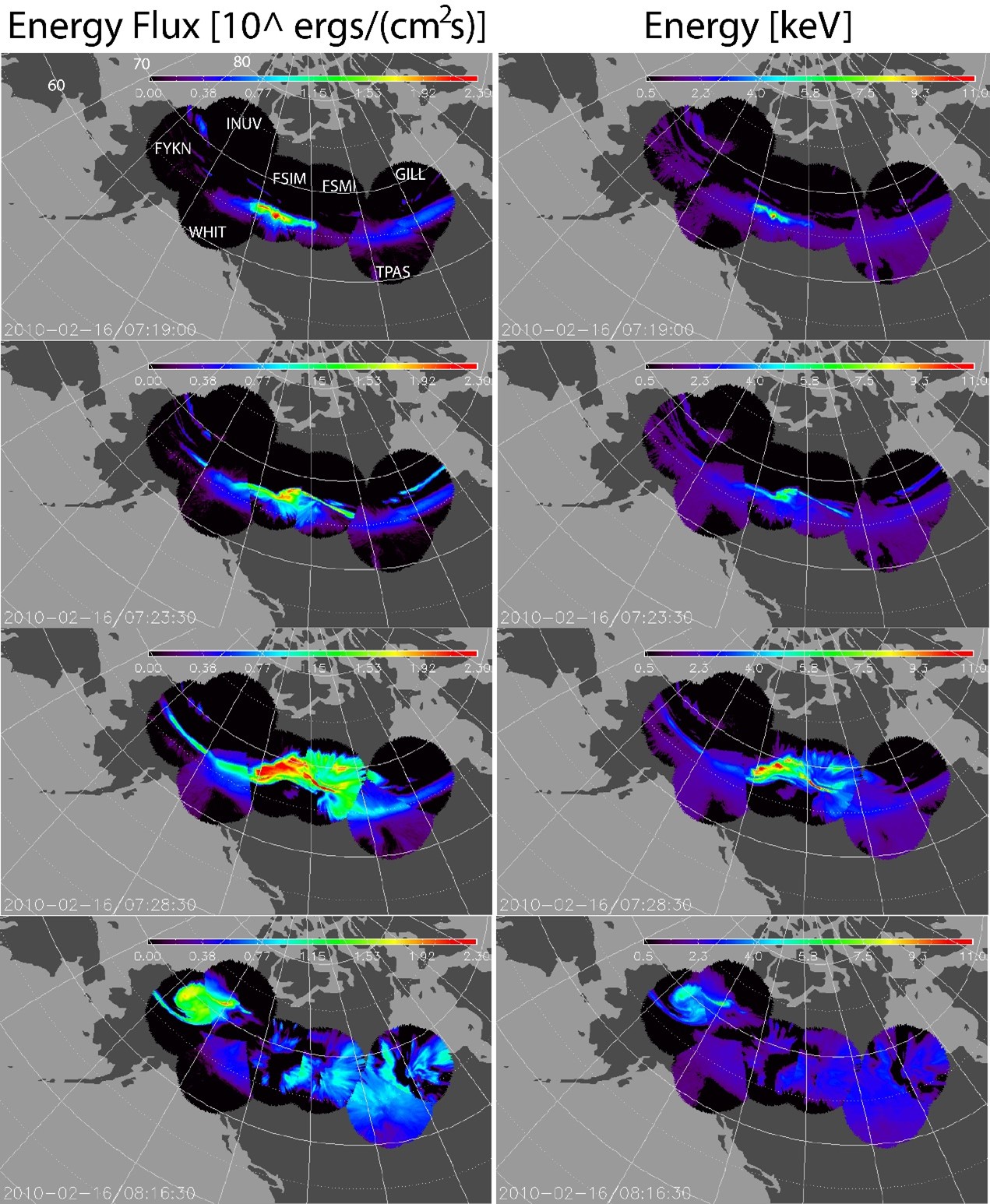
| Figure 1. From Gabrielse et al. (2021), Figure 6. Snapshots in time shortly after substorm onset through substorm poleward expansion and westward traveling surge. Left column: Energy flux (plotted logarithmically) from 1-200 erg cm-2 s-1. Right column: Average energy (plotted linearly) from 0.5-11 keV. Magnetic latitudes and station names are marked in the first panel. |
Methodology
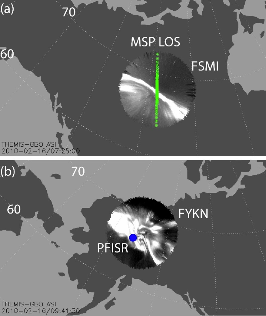
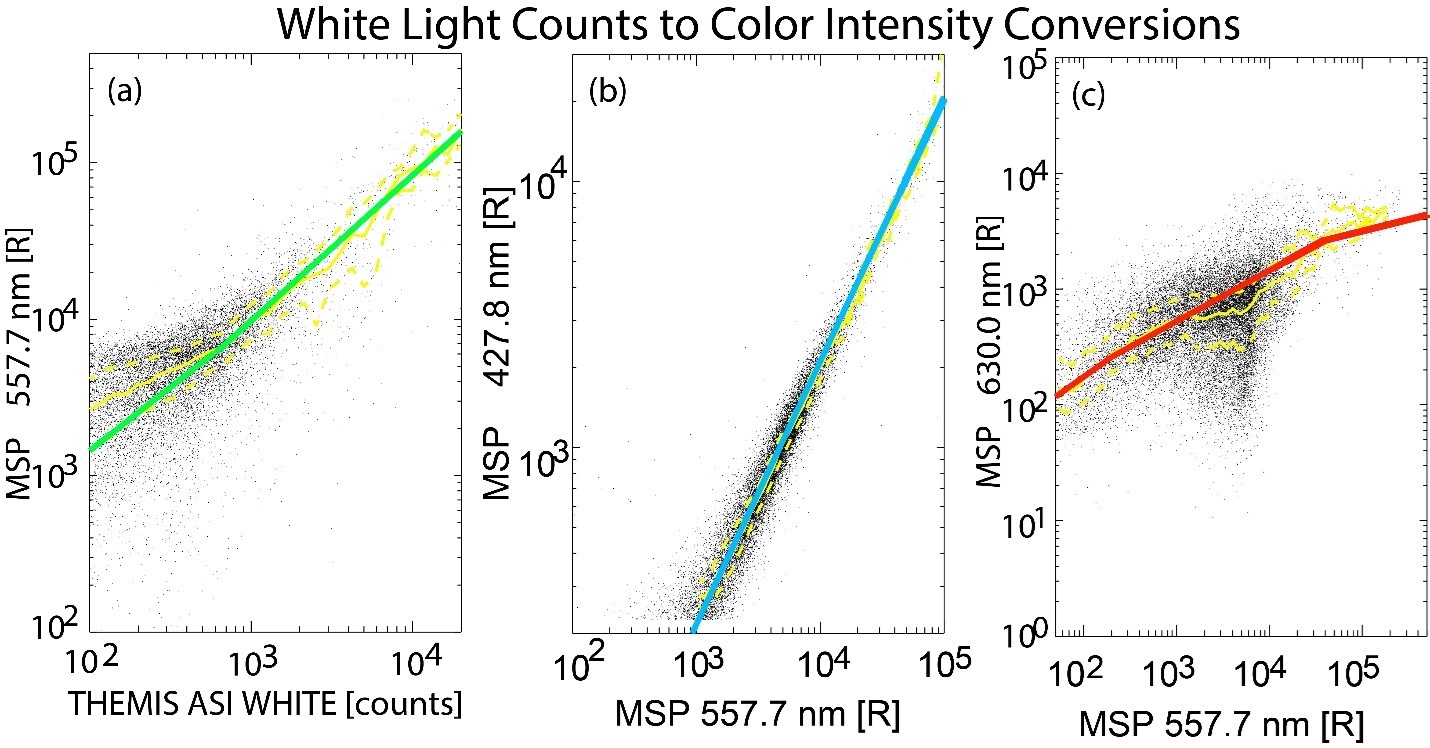
One way to measure the precipitating energy flux and average energy from the aurora is to use the ratio of light intensity between different aurora colors. Because less energetic electrons interact with atmospheric molecules at higher altitudes, they produce the red aurora. More energetic electrons reach lower altitudes and produce the green aurora; even more energetic electrons produce the blue aurora at lower altitudes still. Therefore, aurora that is more energetic will have a higher blue-to-red ratio, whereas a less energetic aurora will have a lower blue-to-red ratio (e.g., Strickland et al., 1989; Hecht et al., 2006; 2008). Using these ratios as inputs to auroral transport codes-in our case, the Boltzmann Three Constituent (B3C) auroral transport code (Strickland et al., 1976; 1993)-both energy flux and average energy can be determined. Because the THEMIS ASIs are white-light cameras, we had to take the first important step to calibrate them with meridian-scanning photometers in order to estimate what those color ratios are. We accomplished this by finding functional fits describing the intensity relationships between the white light and green aurora, as well as the relationships between the blue and green intensities and the red and green intensities. For the color data, we used a meridian scanning photometer (MSP), which collects multispectral wavelengths across latitudes. Figure 2a shows the MSP field of view in green plotted on top of the relevant THEMIS ASI's FOV. Figure 3 shows the scatterplot of data to which we fit analytical functions.
|
| Figure 2. From Gabrielse et al. (2021), Figure 2. (a) Green line depicts the NORSTAR MSP line of sight (LOS) superimposed on top of the THEMIS ASI at Fort Smith, Canada on 2010-02-16 at 07:25 UT. The locations were mapped to 110 km altitude. The white within the ASI FOV is the aurora. Some treetops are visible on the edges of the FOV as black spikes. The stars seen as single white dots are removed in our methodology. (b) The blue dot depicts the PFISR location within the Fort Yukon (FYKN), Canada FOV on 2010-02-16 at 09:41:30 UT. Both panels label the 60° and 70° magnetic latitude lines. |
|
| Figure 3. From Gabrielse et al. (2021), Figure 3. (a) Scatter plot of green light intensity vs. white light counts from 07:00-10:00 UT on 2010-02-16. Solid yellow line shows median whereas dashed yellow lines show quartiles of green intensity for a given white light bin 50 counts wide. The green line represents the functional fit. (b) Scatter plot of blue light intensity vs. green light intensity. Solid yellow line shows median whereas dashed yellow lines show quartiles of blue intensity for a given green light bin 50 R wide. Blue line represents the functional fit. (c) Scatter plot of red light intensity vs. green light intensity. Solid yellow line shows median whereas dashed yellow lines show quartiles of red intensity for a given green light bin 50 R wide. Red line represents the functional fit. |
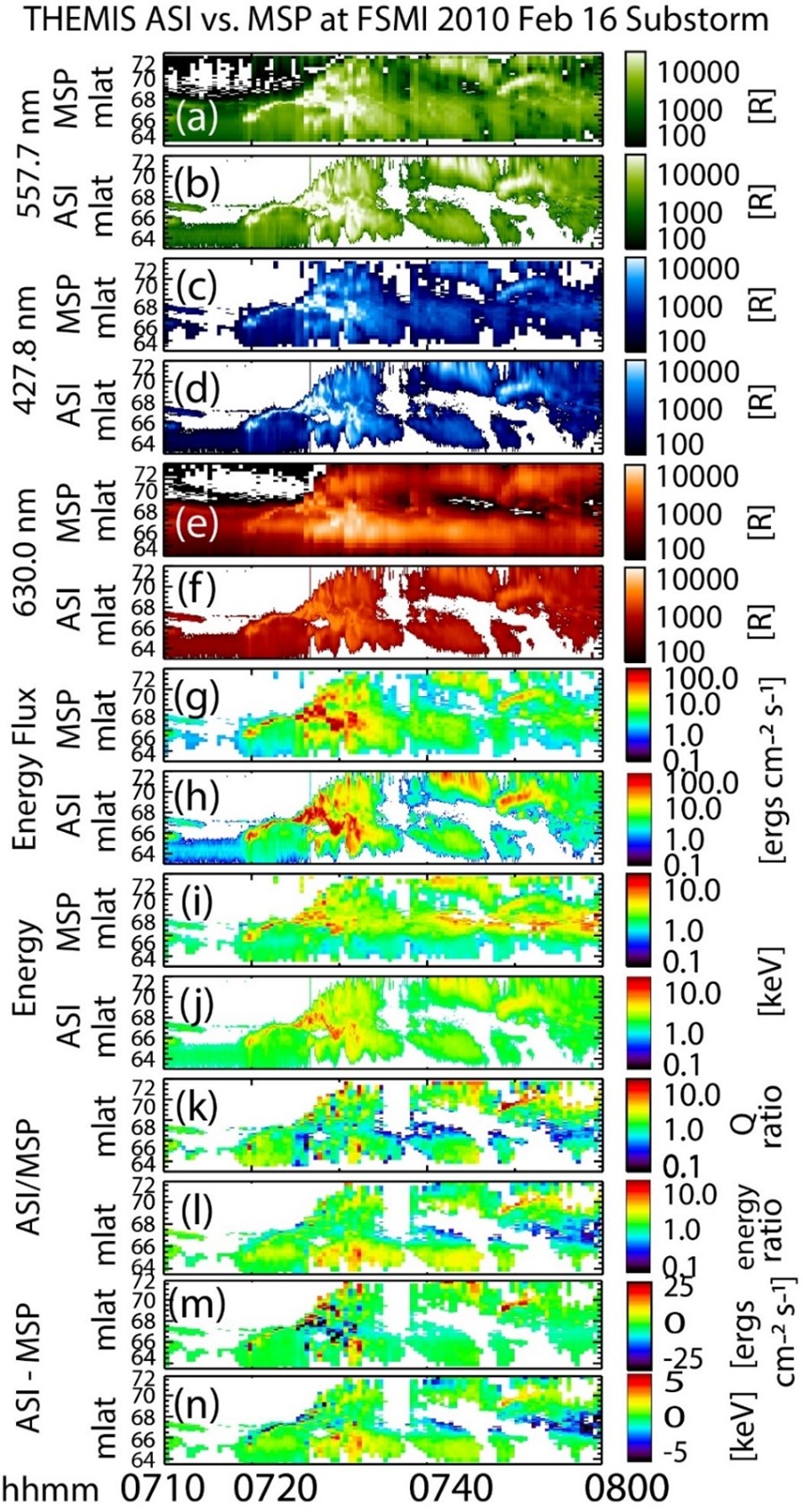
Figure 4 demonstrates the good fit between the colors estimated from the white light intensities and the actual color intensities as measured by the MSP. Gabrielse et al. (2021) includes tables to quantitatively demonstrate the fits. For example, on average, the ASI energy flux underestimates the MSP energy flux by 1.1 erg cm-2 s-1 with a standard deviation of 12.6 erg cm-2 s-1 for the Figure 4 timeframe (07:10-08:00). For the entire calibration time (07:00-10:00), the ASI energy flux underestimates the MSP energy flux by only 0.6 erg cm-2 s-1 on average with a standard deviation of 7.2 erg cm-2 s-1. Furthermore, the average of the ratio of average energies is 1.0, with a median of 0.9 and upper and lower quartiles of 1.2 and 0.6, respectively, for the Figure 4 timeframe.
|
| Figure 4. From Gabrielse et al. (2021), Figure 4. Comparison between MSP data and THEMIS ASI data. Plots are keograms, which display magnetic latitude on the y-axis and time on the x-axis. The visual is therefore the auroral evolution along a single line of longitude over time. (a) MSP 557.7 nm intensity [R]. (b) ASI 557.7 nm intensity [R]. (c) MSP 427.8 nm intensity [R]. (d) ASI 427.8 nm intensity [R]. (e) MSP 630.0 nm intensity [R]. (f) ASI 630.0 nm intensity [R]. (g) MSP determined energy flux using color ratios as input to the B3C-generated look-up table described in section 2.1. (h) ASI determined energy flux using color ratios as input to the B3C-generated look-up table described in section 2.1. (i) MSP-determined energy using color ratios as input to the B3C-generated look-up table described in section 2.1. (j) ASI-determined energy using color ratios as input to the B3C-generated look-up table described in section 2.1. (k) The ratio between ASI (interpolated) and MSP energy fluxes, or panel h divided by panel g. (l) The ratio between ASI (interpolated) and MSP average energies, or panel j divided by panel i. (m) The difference between ASI (interpolated) and MSP energy fluxes, or panel h minus panel g. (n) The difference between ASI (interpolated) and MSP average energies, or panel j minus panel i. |
Results
With the THEMIS ASI 2D capabilities, we were able to ascertain the role that mesoscale aurora plays in the total precipitated energy flux. This is new and exciting since resolving to 100s km scales has previously been out of reach due to data limitations earlier discussed. In this paper, we studied two back-to-back substorms that occurred on February 16, 2010. We found that mesoscale aurora play the largest role during the substorm expansion phase, contributing up to ~80% of the total energy flux immediately after onset and continuing to contribute ~30-55% throughout the remainder of the substorm. The average energy estimated from the ASI mosaic field of view also peaked during the initial expansion phase. Figure 5 shows the contributions of <500 km, <300 km, and <100 km scale sizes in panels (f) and (g). Panels (d) and (e) show the auroral evolution in keogram form for two ASI stations. These data are for the same substorm presented in Figure 1.
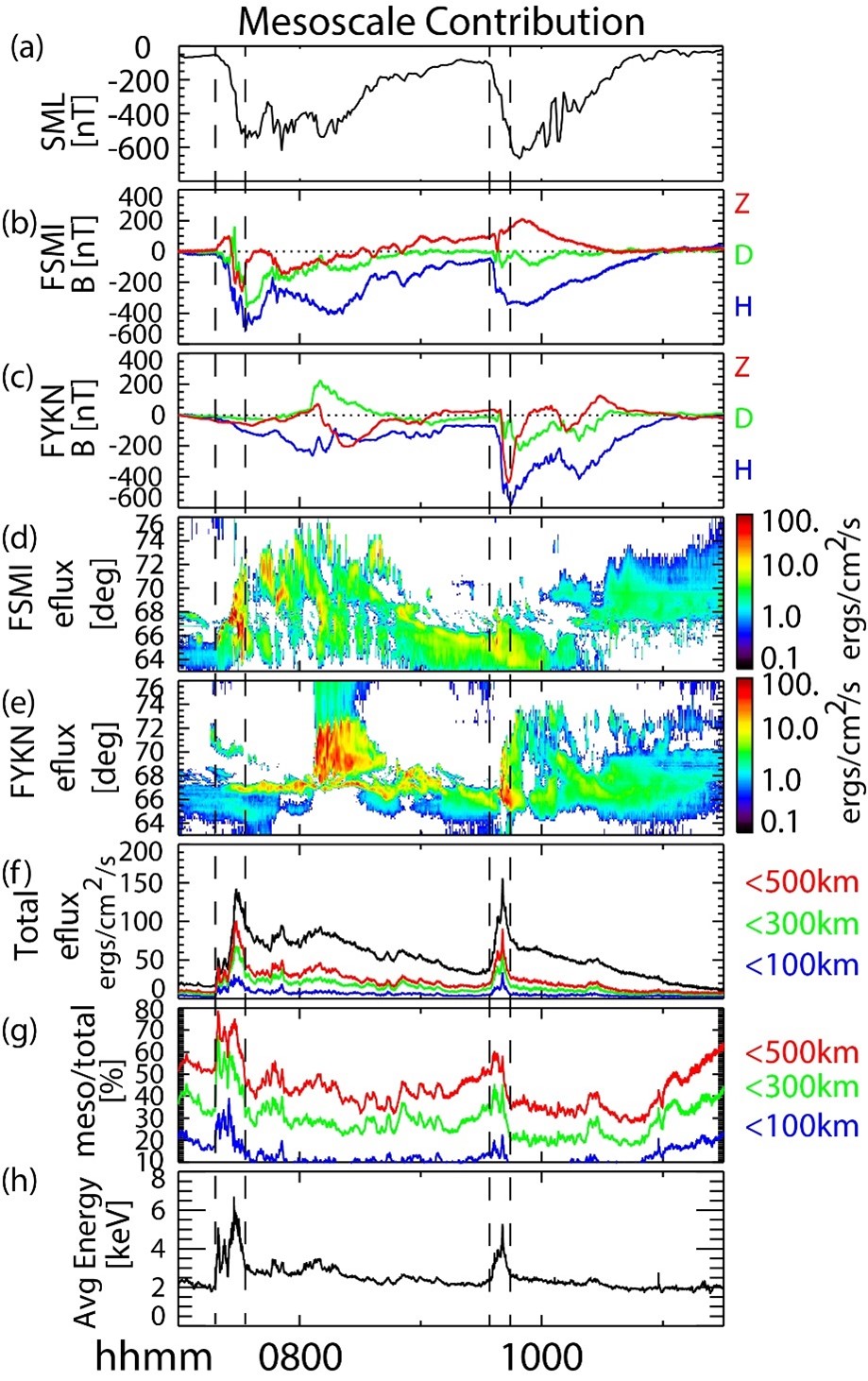
|
| Figure 5. From Gabrielse et al. (2021), Figure 7. (a) SML index (Gjerloev, 2012). (b) Magnetometer data from Fort Smith, near the first substorm onset. (c) Magnetometer data from Fort Yukon, which was closer to the second substorm's onset. (d) Keogram of Fort Smith energy flux. (e) Keogram of Fort Yukon energy flux. (f) Total energy flux observed by the ASI mosaic plotted in black. Total energy flux contributed by scale sizes under 500 km, 300 km and 100 km plotted in red, green, and blue, respectively. (g) Percent of the total energy flux contributed by scale sizes under 500 km, 300 km, and 100 km plotted in red, green, and blue, respectively. (h) Average of the average energy observed over the ASI mosaic. The vertical dashed lines mark the start of the sharp increase in total energy flux and the end of the sharp decrease in total energy flux that occurs during the substorm expansion phase for each substorm (07:18 and 07:33:20 for the first, 09:34:52 and 09:45 UT for the second). |
Lastly, knowing the energy flux and the average energy allowed us to calculate the conductance. These results are also exciting, as current models have been largely limited to producing the conductance from large-scale diffuse aurora. The more dynamic, mesoscale aurora have not been characterized and therefore, the large conductance variations that they cause are left out. We calculated the conductance using the simplistic Robinson formulae, due to its widespread use in the field (for comparisons), as well as with the B3C in order to produce a physically meaningful results. We then compared the values to those obtained from the Poker Flat Incoherent Scatter Radar (PFISR, see Figure 2b), which we took as “ground truth”. Because B3C allows us the choice of a Maxwellian distribution (which describes the diffuse aurora population) or a Gaussian distribution (which describes the discrete aurora population), we plotted both versions and highlight the Gaussian version during discrete aurora (and Maxwellian during diffuse) in Figure 6. Figure 6 shows a very good match between the PFISR Hall conductance and the B3C Hall conductance determined from our THEMIS ASI inputs. Gabrielse et al. (2021) includes tables of various comparative measures, but in summary the Hall conductance as determined by THEMIS-informed B3C and PFISR during discrete aurora has a median percent difference of 24.2% whereas during diffuse aurora the median percent difference is 18.1%.
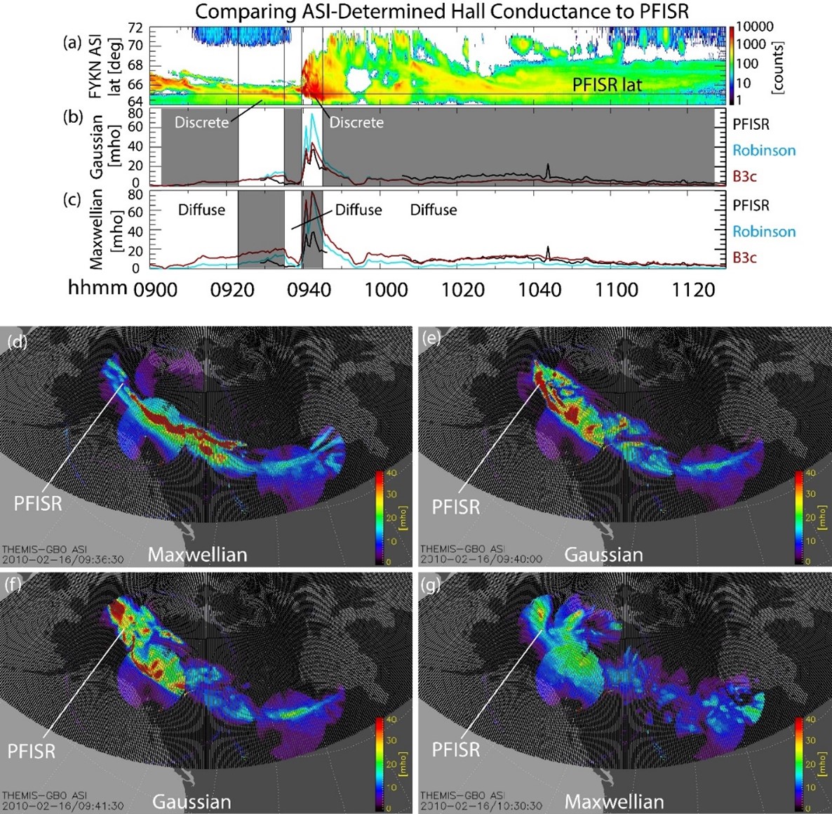
|
| Figure 6. From Gabrielse et al. (2021), Figure 8. Comparing the ASI-determined Hall conductance to PFISR-determined Hall conductance. The discrete and diffuse aurora are marked in panels a-c. The Gaussian distribution was used to determine the conductance related to discrete aurora, and the Maxwellian distribution was used for the diffuse aurora. (a) The FYKN white light intensity keogram at the PFISR longitude. The PFISR latitude line is drawn horizontally. (b) Hall conductance using the Gaussian energy fluxes and average energies from the ASI as input to B3C (red) and Robinson formula (blue) alongside the PFISR-determined result (black). (c) Hall conductance using the Maxwellian energy fluxes and average energies from the ASI as input to B3C (red) and Robinson formula (blue) alongside the PFISR-determined result (black). (d) 2D snapshot of Hall conductance assuming a Maxwellian distribution at 09:36:30 UT. (e) 2D snapshot of Hall conductance assuming a Gaussian distribution at 09:40:00. (f) 2D snapshot of Hall conductance assuming a Gaussian distribution at 09:41:30. (g) 2D snapshot of Hall conductance assuming a Maxwellian distribution at 10:30:30 UT. |
Conclusion
This paper presented a new methodology to utilize the mosaic of THEMIS all-sky-imagers to study auroral precipitation in 2D over time, estimating parameters such as energy flux, average energy, and Hall conductance. Using two consecutive substorms for a case study, results demonstrated the importance of mesoscale auroral forms (10s km to 500 km scale sizes) to the overall energy flux deposition to the ionosphere, particularly during the initial expansion phase immediately after onset. Mesoscale aurora contributed up to ~80% (~60%) of the total energy flux immediately after onset during the early expansion phase of the first (second) substorm, and continued to contribute ~30-55% throughout the remainder of the substorm. Because prior work highly relied upon statistics, the mesoscale contribution has not been so well-resolved before, especially for specific case studies. The results indicate the importance of including mesoscale auroral forms in global models to appropriately capture the related physics. Additionally, the paper demonstrated the 2D time series data product that can be provided to modelers when ASI data are available, allowing for case-specific data-informed modeling. The methods showed a good comparison between the calibrated ASI data and the MSP data. As expected, the greatest scatter is in 630.0 nm wavelength. As a future work, the redline ASI cameras that are currently coming online as part of the TREx array of ASIs could be used to specify the 630.0 nm wavelength more accurately (https://www.ucalgary.ca/aurora/projects/trex). Comparing and/or calibrating to DMSP energy fluxes and average energies would also provide additional information on the uncertainties and/or improve our estimates. The Hall conductance was well-captured by the B3C auroral transport code informed by ASI energy fluxes and average energies, when compared to PFISR-determined Hall conductance. The ASI-informed Robinson formula overestimated the Hall conductance during discrete aurora and underestimated during diffuse aurora.
References
Burch, J. L., Mende, S. B., Mitchell, D. G., Moore, T. E., Pollock, C. J., Reinisch, B. W., Sandel, B. R., Fuselier, S. A., Gallagher, D. L., Green, J. L., Perez, J. D., Reiff, P. H., (2001), Views of Earth's Magnetosphere with the IMAGE Satellite, Science, 291 (5504), 619-624, doi: 10.1126/science.291.5504.619.Deng, Y., Heelis, R., Lyons, L. R., Nishimura, Y., & Gabrielse, C. (2019). Impact of flow bursts in the auroral zone on the ionosphere and thermosphere. Journal of Geophysical Research: Space Physics, 124,https://doi.org/10.1029/2019JA026755
Gabrielse C., T. Nishimura, M. Chen, J. H. Hecht, S. R. Kaeppler, D. M. Gillies, A. S. Reimer, L. R. Lyons, Y. Deng, E. Donovan and J. S. Evans (2021), Estimating Precipitating Energy Flux, Average Energy, and Hall Auroral Conductance From THEMIS All-Sky-Imagers With Focus on Mesoscales, Frontiers in Physics, Vol 9, DOI: 10.3389/fphy.2021.744298, https://www.frontiersin.org/article/10.3389/fphy.2021.744298
Acknowledgments
The work in this paper was gratefully funded by NASA grants 80NSSC20K0725, 80NSSC18K0657, 80NSSC20K0604, 80NSSC20K0195, and 80NSSC20K1786, AFOSR Grant FA9559 –16 –1 –0364, and NSF grants AGS 1602862 and AGS-1907698. The THEMIS mission is supported by NASA contract NAS5-02099, NSF grant AGS-1004736, and CSA contract 9F007-046101. This material is based upon work supported by the Poker Flat Incoherent Scatter Radar which is a major facility funded by the National Science Foundation through cooperative agreement AGS-1840962 to SRI International. We gratefully acknowledge the SuperMAG collaborators (Link). The ASI, PFISR and SuperMAG data are available at themis.ssl.berkeley.edu, isr.sri.com/madrigal, and supermag.jhuapl.edu.
 Please send comments/suggestions to
Emmanuel Masongsong / emasongsong @ igpp.ucla.edu
Please send comments/suggestions to
Emmanuel Masongsong / emasongsong @ igpp.ucla.edu